Spark Window Functions for DataFrames and SQL

Introduced in Spark 1.4, Spark window functions improved the expressiveness of Spark DataFrames and Spark SQL. With window functions, you can easily calculate a moving average or cumulative sum, or reference a value in a previous row of a table. Window functions allow you to do many common calculations with DataFrames, without having to resort to RDD manipulation.

Aggregates, UDFs vs. Window functions

Window functions are complementary to existing DataFrame operations: aggregates, such as sum and avg, and UDFs. To review, aggregates calculate one result, a sum or average, for each group of rows, whereas UDFs calculate one result for each row based on only data in that row. In contrast, window functions calculate one result for each row based on a window of rows. For example, in a moving average, you calculate for each row the average of the rows surrounding the current row; this can be done with window functions.

Moving Average Example

Let us dive right into the moving average example. In this example dataset, there are two customers who have spent different amounts of money each day.

// Building the customer DataFrame. All examples are written in Scala with Spark 1.6.1, but the same can be done in Python or SQL.

val customers = sc.parallelize(List(("Alice", "2016-05-01", 50.00),

                                    ("Alice", "2016-05-03", 45.00),

                                    ("Alice", "2016-05-04", 55.00),

                                    ("Bob", "2016-05-01", 25.00),

                                    ("Bob", "2016-05-04", 29.00),

                                    ("Bob", "2016-05-06", 27.00))).

                               toDF("name", "date", "amountSpent")

// Import the window functions.

import org.apache.spark.sql.expressions.Window

import org.apache.spark.sql.functions._

// Create a window spec.

val wSpec1 = Window.partitionBy("name").orderBy("date").rowsBetween(-1, 1)

In this window spec, the data is partitioned by customer. Each customer’s data is ordered by date. And, the window frame is defined as starting from -1 (one row before the current row) and ending at 1 (one row after the current row), for a total of 3 rows in the sliding window.

// Calculate the moving average

customers.withColumn( "movingAvg",

                                             avg(customers("amountSpent")).over(wSpec1)  ).show()

This code adds a new column, “movingAvg”, by applying the avg function on the sliding window defined in the window spec:

name	date	amountSpent	movingAvg
Alice	5/1/2016	50	47.5
Alice	5/3/2016	45	50
Alice	5/4/2016	55	50
Bob	5/1/2016	25	27
Bob	5/4/2016	29	27
Bob	5/6/2016	27	28

Window function and Window Spec definition

As shown in the above example, there are two parts to applying a window function: (1) specifying the window function, such as avg in the example, and (2) specifying the window spec, or wSpec1 in the example. For (1), you can find a full list of the window functions here:
https://spark.apache.org/docs/latest/api/scala/index.html#org.apache.spark.sql.functions$
 You can use functions listed under “Aggregate Functions” and “Window Functions”.

For (2) specifying a window spec, there are three components: partition by, order by, and frame.

1.     “Partition by” defines how the data is grouped; in the above example, it was by customer. You have to specify a reasonable grouping because all data within a group will be collected to the same machine. Ideally, the DataFrame has already been partitioned by the desired grouping.
2.       “Order by” defines how rows are ordered within a group; in the above example, it was by date.
3.       “Frame” defines the boundaries of the window with respect to the current row; in the above example, the window ranged between the previous row and the next row.

Cumulative Sum

Next, let us calculate the cumulative sum of the amount spent per customer.

// Window spec: the frame ranges from the beginning (Long.MinValue) to the current row (0).

val wSpec2 = Window.partitionBy("name").orderBy("date").rowsBetween(Long.MinValue, 0)

// Create a new column which calculates the sum over the defined window frame.

customers.withColumn( "cumSum",

  sum(customers("amountSpent")).over(wSpec2)  ).show()

name	date	amountSpent	cumSum
Alice	5/1/2016	50	50
Alice	5/3/2016	45	95
Alice	5/4/2016	55	150
Bob	5/1/2016	25	25
Bob	5/4/2016	29	54
Bob	5/6/2016	27	81

Data from previous row

In the next example, we want to see the amount spent by the customer in their previous visit.

// Window spec. No need to specify a frame in this case.

val wSpec3 = Window.partitionBy("name").orderBy("date")

// Use the lag function to look backwards by one row.

customers.withColumn("prevAmountSpent",

 lag(customers("amountSpent"), 1).over(wSpec3) ).show()

name	date	amountSpent	prevAmountSpent
Alice	5/1/2016	50	null
Alice	5/3/2016	45	50
Alice	5/4/2016	55	45
Bob	5/1/2016	25	null
Bob	5/4/2016	29	25
Bob	5/6/2016	27	29

Rank

In this example, we want to know the order of a customer’s visit (whether this is their first, second, or third visit).

// The rank function returns what we want.

customers.withColumn( "rank", rank().over(wSpec3) ).show()

name	date	amountSpent	rank
Alice	5/1/2016	50	1
Alice	5/3/2016	45	2
Alice	5/4/2016	55	3
Bob	5/1/2016	25	1
Bob	5/4/2016	29	2
Bob	5/6/2016	27	3

Conclusion

I hope these examples have helped you understand Spark’s window functions. There is more functionality that was not covered here. To learn more, please see the Databricks article on this topic: https://databricks.com/blog/2015/07/15/introducing-window-functions-in-spark-sql.html

Introduction to Spark for Developers and Data Scientists

What is Spark?

Spark is “a fast and general engine for large-scale data processing”. – http://spark.apache.org/

Spark is also one of the most popular open source frameworks for big data, based on number of contributors. Let us find out why this is the case.

When do you use Spark?

Suppose you would like to analyze a data set: perform ETL or data munging, then run SQL queries such as grouping and aggregations against the data, and maybe apply a machine learning algorithm. When the data size is small, everything will run quickly on a single machine, and you can use analysis tools like Pandas (Python), R, or Excel, or write your own scripts. But, for larger data sets, data processing will be too slow on a single machine, and then you will want to move to a cluster of machines. This is when you would use Spark.

You could probably benefit from Spark if:

•       Your data is currently stored in Hadoop / HDFS.
•       Your data set contains more than 100 million rows.
•       Ad-hoc queries take longer than 5 minutes to complete.

What Spark is Not, typical architecture

Spark can be a central component to a big data system, but it is not the only component. It is not a distributed file system: you would typically store your data on HDFS or S3. Nor is Spark a NoSQL database: Cassandra or HBase would be a better place for horizontally scalable table storage. And, it is not a message queue: you would use Kafka or Flume to collect streaming event data. Spark is, however, a compute engine which can take input or send output to all of these other systems.

How do you use Spark?

Implemented in Scala, Spark can be programmed in Scala, Java, Python, SQL, and R. However, not all of the latest functionality is immediately available in all languages.

What kind of operations does Spark support?

Spark SQL. Spark supports batch operations involved in ETL and data munging, via the DataFrame API. It supports parsing different input formats, such as JSON or Parquet. Once the raw data is loaded, you can easily compute new columns from existing columns. You can slice and dice the data by filtering, grouping, aggregating, and joining with other tables. Spark supports relational queries, which you can express in SQL or through the DataFrame API.

Spark Streaming. Spark also provides scalable stream processing. Given an input data stream, for example, coming from Kafka, Spark allows you to perform operations on the streaming data, such as map, reduce, join, and window.

MLlib. Spark includes a machine learning library, with scalable algorithms for classification, regression, collaborative filtering, clustering, and more. If training your dataset on a single machine takes too long, you might consider cluster computing with Spark.

GraphX. Finally, GraphX is a component in Spark for scalable batch processing on graphs.

As you may have noticed by now, Spark processing is batch oriented. It works best when you want to perform the same operation on all of your data, or a large subset of your data. Even with Spark Streaming, you operate on small batches of the data stream, rather than one event at a time.

Spark vs. Hadoop MapReduce, Hive, Impala

How does Spark compare with other big data compute engines? Unlike Hadoop MapReduce, Spark caches data in memory for huge performance gains when you have ad-hoc queries or iterative workloads, which are common in machine learning algorithms. Hive and Impala both run SQL queries at scale; the advantage of Spark over these systems is (1) the convenience of writing both queries and UDFs in the same language, such as Scala, and (2) support for machine learning algorithms, streaming data, and graph processing within the same system.

Conclusion

This overview has explained what Spark is, when to use it, what kinds of operations it supports, and how it compares with other big data systems. To learn more, please take a look at the Spark website (http://spark.apache.org/).

Spark 1.6 Datasets API: Example Usage

Overview

Spark 1.6 introduced a new Datasets API. It is an extension of Dataframes that supports functional processing on a collection of objects. Let's take a look at some examples of how to use them. First we'll read a JSON file and a text file into Datasets. We will apply functional transformations to parse the data. Then we will run relational queries against a Dataset.

Creating a Dataset from a JSON file

Suppose you have JSON formatted data which you would like to read into a Dataset. Here is an example JSON file:

Contents of "students.json" --

{"name":"Alice", "dept":"Math"}
{"name":"Bob", "dept":"CS"}
{"name":"Carl", "dept":"Math"}

To create a Dataset from this JSON file:

// Define the Student row type.
> case class Student(name: String, dept: String)
// Read JSON objects into a Dataset[Student].
> val studentsFromJSON = sqlContext.read.json("students.json").as[Student]

Creating a Dataset from a Text file

Suppose instead you have data in a text file, in tab-separated (.tsv) format:

Alice<tab>Math<tab>18
Bob<tab>CS<tab>19
Carl<tab>Math<tab>21

To create a Dataset from this text file:

// Read the lines of the file into a Dataset[String].
> val studentsFromText = sqlContext.read.text("students.tsv").as[String]

(result) studentsFromText: org.apache.spark.sql.Dataset[String] = [value: string]

// We want a Dataset of type "Student".
case class Student(name: String, dept: String, age:Int)

// Functional programming to parse the lines into a Dataset[Student].

val students = studentsFromText.
  map(line => {

    val cols = line.split("\t") // parse each line

    Student(cols(0), cols(1), cols(2).toInt)

  })

(result) students: org.apache.spark.sql.Dataset[Student] = [name: string, dept: string, age: int]

// Show the contents of the Dataset.

> students.show()

| name|dept|age|

+-----+----+---+

|Alice|Math| 18|

|  Bob|  CS| 19|

| Carl|Math| 21|

Relational queries

Datasets support relational queries, with operations such as: select, filter, group by, count, avg, join.

SELECT, FILTER

Get the names of students in the Math department.

// Select two columns and filter on one column.
// Each argument of "select" must be a "TypedColumn".

> students.select($"name".as[String], $"dept".as[String]).

    filter(_._2 == "Math").  // Filter on _2, the second selected column

    collect()

(result) Array((Alice,Math), (Carl,Math))

GROUP BY, COUNT

Count the number of students in each department.

// Group by department and count each group.

> students.groupBy(_.dept).count().collect()

(result) Array((CS,1), (Math,2))

GROUP BY, AVG

Average age in each department.

// Import the "avg" function.

> import org.apache.spark.sql.functions._

// Group and aggregate in each group.

> students.groupBy(_.dept).
    agg(avg($"age").as[Double]).
    collect()

(result) Array((CS,19.0), (Math,19.5))

JOIN

Suppose we have a separate table with deparment information. We would like to join the department information into our student table.

First, create the department Dataset.

// The Department type.

> case class Department(abbrevName: String, fullName: String)

// Initialize a Seq and convert to a Dataset.

> val depts = Seq(Department("CS", "Computer Science"), Department("Math", "Mathematics")).toDS()

// Show the contents of the Dataset.

> depts.show()

|abbrevName|        fullName|

+----------+----------------+

|        CS|Computer Science|

|      Math|     Mathematics|

Join the students Dataset with the departments Dataset.

// Join two datasets with "joinWith".

> val joined = students.joinWith(depts, $"dept" === $"abbrevName")

// Show the contents of the joined Dataset.
// Note that the original objects are nested into tuples under the _1 and _2 columns.

> joined.show()

|             _1|                  _2|

+---------------+--------------------+

|[Alice,Math,18]|  [Math,Mathematics]|

|    [Bob,CS,19]|[CS,Computer Scie...|

| [Carl,Math,21]|  [Math,Mathematics]|

Select two columns from the joined Dataset.

// Use "map" to select from the joined Dataset. 
// Notice that the original Dataset types are preserved.

> joined.map(s => (s._1.name, s._2.fullName)).show()

|   _1|              _2|

+-----+----------------+

|Alice|     Mathematics|

|  Bob|Computer Science|

| Carl|     Mathematics|

EXPLAIN

"Explain" prints the query's physical plan for debugging.

// Explain how the join is computed.
// Note that a BroadcastJoin is planned.
> joined.explain()

== Physical Plan ==

Project [struct(name#168163,dept#168164,age#168165) AS _1#168203,struct(abbrevName#168200,fullName#168201) AS _2#168204]

+- BroadcastHashJoin [dept#168164], [abbrevName#168200], BuildRight

   :- ConvertToUnsafe

   :  +- !MapPartitions <function1>, class[value[0]: string], class[name[0]: string, dept[0]: string, age[0]: int], [name#168163,dept#168164,age#168165]

   :     +- ConvertToSafe

   :        +- Scan TextRelation[value#168157] InputPaths: /students.tsv

   +- ConvertToUnsafe

      +- LocalTableScan [abbrevName#168200,fullName#168201], [[0,1800000002,2000000010,5343,72657475706d6f43,65636e6569635320],[0,1800000004,200000000b,6874614d,74616d656874614d,736369]]

References

Spark API docs: http://spark.apache.org/docs/latest/api/scala/index.html#org.apache.spark.sql.Dataset

Spark Programming Guide: http://spark.apache.org/docs/latest/sql-programming-guide.html

Introducing Spark Datasets: https://databricks.com/blog/2016/01/04/introducing-spark-datasets.html

Grace Hopper Conference 2015 Wrap up

Very briefly, highlights from GHC 2015 ...

Susan Wojcicki's (CEO of Youtube) keynote speech. She talked about two reasons why there are so few women in tech: (1) not enough women in the pipeline, starts in elementary / middle school, and (2) retention of women in tech - a workplace culture that causes women to leave at twice the rate of men. Not enough support for maternity leave and working moms is a problem. Her career advice: "Keep asking to be invited." "Power and influence is passed down from those who have it."

Clara Shih, CEO of Hearsay Social offers career advice: (1) embrace failure, (2) nurture relationships.

Manuela Veloso's (CMU) keynote on symbiotic autonomy for autonomous robots. Robots can navigate around buildings with the help of humans.

Dinner with Duy Loan Le, former TI fellow, and Vietnamese Women in Computing. Follow your own path; don't compare yourself to others. Fail fast. It was nice meeting other Vietnamese women in computing.

My birds-of-a-feather discussion on maternity leave. There were lots of good conversations about fitting maternity leave into a woman's career. Key take aways: (1) ask for what you need, (2) start building your network now.

Lunch time table topic: Asian American identity in computing. Intersectionality.

All the conversations I had with women from other companies and students. Catching up with former co-workers.

Anita Borg Institute: you belong (in this field).

Hour of Code: teaching computer science in public schools is the best way to increase diversity in CS.

Jo Miller career workshop: for leaders, "delivers results" is a must-have.

What worked: meet your friend's friends: I met so many women through my former co-worker. Lunch time table topics lead to interesting conversations. Speaking at the conference is a great way to be involved. I had good conversations with people sitting next to me at talks.

For next time (if there is a next time): talk with more students. Stay for the full conference: more time to network. Most technical talks are beginner level, so go to talks to learn something new, and not on topics you already know. After meeting someone, always get their name and / or business card. Stay in lodging as close to the conference as possible. Don't do work if possible.

Attending Grace Hopper Conference

I will be attending the Grace Hopper Celebration of Women in Computing this October, in Houston, TX. I am looking forward to connecting with other women in data science and big data. I would love to compare notes on Spark, Scala, Databricks, and machine learning. I would also like to meet others doing agile and scrum, or leading data science projects. There will be talks on professional development, and I will be leading a discussion on the impact of maternity leave on a woman's career. Last, but not least, I will be happy to discuss jobs at Samsung SDSA with job seekers.

Reading JSON data in Spark DataFrames

Overview

Spark DataFrames makes it easy to read from a variety of data formats, including JSON. In fact, it even automatically infers the JSON schema for you. Once the data is loaded, however, figuring out how to access individual fields is not so straightforward. This post will walk through reading top-level fields as well as JSON arrays and nested objects. The code provided is for Spark 1.4. Update: please see my updated post on an easier way to work with nested array of struct JSON data.

Load the JSON File

Let's begin by loading a JSON file, where each line is a JSON object:

{"name":"Michael", "cities":["palo alto", "menlo park"], "schools":[{"sname":"stanford", "year":2010}, {"sname":"berkeley", "year":2012}]}

{"name":"Andy", "cities":["santa cruz"], "schools":[{"sname":"ucsb", "year":2011}]}

{"name":"Justin", "cities":["portland"], "schools":[{"sname":"berkeley", "year":2014}]}

The Scala code to read a JSON file:

>> val people = sqlContext.read.json("people.json")

people: org.apache.spark.sql.DataFrame

Read a Top-Level Field

With the above command, all of the data is read into a DataFrame. In the following examples, I will show how to extract individual fields into arrays of primitive types. Let's start with the top-level "name" field:

>> val names = people.select('name).collect()

names: Array[org.apache.spark.sql.Row] = Array([Michael], [Andy], [Justin])

>> names.map(row => row.getString(0))

res88: Array[String] = Array(Michael, Andy, Justin)

Use the select() method to specify the top-level field, collect() to collect it into an Array[Row], and the getString() method to access a column inside each Row.

Flatten and Read a JSON Array

Update: please see my updated post on an easier way to work with nested array of struct JSON data.

Next, notice that each Person has an array of "cities". Let's flatten these arrays and read out all their elements.

>> val flattened = people.explode("cities", "city"){c: List[String] => c}

flattened: org.apache.spark.sql.DataFrame

>> val allCities = flattened.select('city).collect()

allCities: Array[org.apache.spark.sql.Row]

>> allCities.map(row => row.getString(0))

res92: Array[String] = Array(palo alto, menlo park, santa cruz, portland)

The explode() method explodes, or flattens, the cities array into a new column named "city". We then use select() to select the new column, collect() to collect it into an Array[Row], and getString() to access the data inside each Row.

Read an Array of Nested JSON Objects, Unflattened

Finally, let's read out the "schools" data, which is an array of nested JSON objects. Each element of the array holds the school name and year:

>> val schools = people.select('schools).collect()

schools: Array[org.apache.spark.sql.Row]

>> val schoolsArr = schools.map(row => row.getSeq[org.apache.spark.sql.Row](0))

schoolsArr: Array[Seq[org.apache.spark.sql.Row]]

>> schoolsArr.foreach(schools => {

>>    schools.map(row => print(row.getString(0), row.getLong(1)))

>>    print("\n")

>> })

(stanford,2010)(berkeley,2012) 

(ucsb,2011) 

(berkeley,2014)

Use select() and collect() to select the "schools" array and collect it into an Array[Row]. Now, each "schools" array is of type List[Row], so we read it out with the getSeq[Row]() method. Finally, we can read the information for each individual school, by calling getString() for the school name and getLong() for the school year. Phew!

Summary

In this blog post, we have walked through accessing top-level fields, arrays, and nested JSON objects from JSON data. The key classes involved were DataFrame, Array, Row, and List. We used the select(), collect(), and explode() DataFrame methods, and the getString(), getLong(), and get Seq[T]() Row methods to read data out into arrays of primitive types.

GraphX: Graph Computing for Spark

Overview

I've been reading about GraphX, Spark's graph processing library. GraphX provides distributed, in-memory graph computing. The key thing that differentiates it from other large-scale graph processing sytems, like Giraph and GraphLab, is that it is tightly integrated within the Spark ecosystem. This allows efficient data pipelines that combine ETL (SQL), machine learning, and graph analysis within one framework (Spark), without the overhead of running multiple systems and copying data between them.

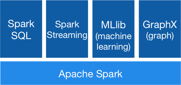
The Spark stack.

Graph Library for the Spark Framework

Graphs in GraphX are directed multigraph property graphs, which means that each vertex and each edge can have properties (attributes) associated with it. GraphX graphs are distributed and immutable. You create a graph in GraphX by providing an RDD of vertices and an RDD of edges. You can then perform OLAP operations on a graph through the API. A pregel API supports vertex-centric, bulk-synchronous parallel, iterative algorithms.

In-memory indexes speed up graph operations. Edge partitioning (which means vertices can be split across partitions) and vertex data replication speed up edge traversal, which usually involves communication across machines. A 2014 research paper shows performance comparable to other graph systems, Giraph and GraphLab.

GraphX is built on RDDs.

Applications

A couple of recent MLLib algorithms are implemented on GraphX: LDA topic modeling and Power Iteration Clustering. Alibaba Taobao uses GraphX for data mining in ecommerce, modeling user-item-merchant interactions as a graph. Netflix uses GraphX for movie recommendation, with graph diffusion and LDA clustering algorithms.